Graph
This section of the user guide covers the syntax and theory behind graph expressions. Examples are presented for two key graph use cases: bipartite graph recommenders and event correlation with temporal graph queries.
Graphs
Log records and other data indexed in Solr have connections between them that can be seen as a distributed graph. Graph expressions provide a mechanism for identifying root nodes in the graph and walking their connections. The general goal of the graph walk is to materialize a specific subgraph and perform link analysis to understand the connections between nodes.
In the next few sections below we’ll review the graph theory behind Solr’s graph expressions.
Subgraphs
A subgraph is a smaller subset of the nodes and connections of the larger graph. Graph expressions allow you to flexibly define and materialize a subgraph from the larger graph stored in the distributed index.
Subgraphs play two important roles:
-
They provide a local context for link analysis. The design of the subgraph defines the meaning of the link analysis.
-
They provide a foreground graph that can be compared to the background index for anomaly detection purposes.
Bipartite Subgraphs
Graph expressions can be used to materialize bipartite subgraphs. A bipartite graph is a graph where the nodes are split into two distinct categories. The links between those two categories can then be analyzed to study how they relate. Bipartite graphs are often discussed in the context of collaborative filter recommender systems.
A bipartite graph between shopping baskets and products is a useful example. Through link analysis between the shopping baskets and products we can determine which products are most often purchased within the same shopping baskets.
In the example below there is a Solr collection called baskets with three fields:
id: Unique ID
basket_s: Shopping basket ID
product_s: Product
Each record in the collection represents a product in a shopping basket. All products in the same basket share the same basket ID.
Let’s consider a simple example where we want to find a product that is often sold with butter. In order to do this we could create a bipartite subgraph of shopping baskets that contain butter. We won’t include butter itself in the graph as it doesn’t help with finding a complementary product for butter.
Below is an example of this bipartite subgraph represented as a matrix:
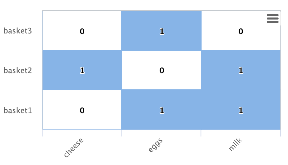
In this example there are three shopping baskets shown by the rows: basket1, basket2, basket3.
There are also three products shown by the columns: cheese, eggs, milk.
Each cell has a 1 or 0 signifying if the product is in the basket.
Let’s look at how Solr graph expressions materializes this bipartite subgraph:
The nodes function is used to materialize a subgraph from the larger graph.
Below is an example nodes function which materializes the bipartite graph shown in the matrix above.
nodes(baskets,
      random(baskets, q="product_s:butter", fl="basket_s", rows="3"),
      walk="basket_s->basket_s",
      fq="-product_s:butter",
      gather="product_s",
      trackTraversal="true")
Let’s break down this example starting with the random function:
random(baskets, q="product_s:butter", fl="basket_s", rows="3")The random function is searching the baskets collection with the query product_s:butter, and
returning 3 random samples.
Each sample contains the basket_s field which is the basket id.
The three basket id’s that are returned by the random sample are the root nodes of the graph query.
The nodes function is the graph query.
The nodes function is operating over the three root nodes returned
by the random function.
It "walks" the graph by searching the basket_s field of the root nodes against the basket_s field in the index.
This finds all the product records for the root baskets.
It will then "gather" the product_s field from the records it finds in the walk.
A filter is applied so that records with butter in the product_s field will not be returned.
The trackTraversal flag tells the nodes expression to track the links between the root baskets and products.
Node Sets
The output of the nodes function is a node set that represents the subgraph specified by the nodes function.
The node set contains a unique set of nodes that are gathered during the graph walk.
The node property in the result is the value of the gathered node.
In the shopping basket example the product_s field is in the node property because that was what was specified to be gathered in the nodes expression.
The output of the shopping basket graph expression is as follows:
{
  "result-set": {
    "docs": [
      {
        "node": "eggs",
        "collection": "baskets",
        "field": "product_s",
        "ancestors": [
          "basket1",
          "basket3"
        ],
        "level": 1
      },
      {
        "node": "cheese",
        "collection": "baskets",
        "field": "product_s",
        "ancestors": [
          "basket2"
        ],
        "level": 1
      },
      {
        "node": "milk",
        "collection": "baskets",
        "field": "product_s",
        "ancestors": [
          "basket1",
          "basket2"
        ],
        "level": 1
      },
      {
        "EOF": true,
        "RESPONSE_TIME": 12
      }
    ]
  }
}
The ancestors property in the result contains a unique, alphabetically sorted set of all the inbound links to the node in the subgraph.
In this case it shows the baskets that are linked to each product.
The ancestor links will only be tracked when the trackTraversal flag is turned on in the nodes expression.
Link Analysis and Degree Centrality
Link analysis is often performed to determine node centrality. When analyzing for centrality the goal is to assign a weight to each node based on how connected it is in the subgraph. There are different types of node centrality. Graph expressions very efficiently calculates inbound degree centrality (in-degree).
Inbound degree centrality is calculated by counting the number of inbound links to each node. For simplicity this document will sometimes refer to inbound degree simply as degree.
Back to the shopping basket example:
We can calculate the degree of the products in the graph by summing the columns:
cheese: 1
eggs:   2
milk:   2
From the degree calculation we know that eggs and milk appear more frequently in shopping baskets with butter than cheese does.
The nodes function can calculate degree centrality by adding the count(*) aggregation as shown below:
nodes(baskets,
      random(baskets, q="product_s:butter", fl="basket_s", rows="3"),
      walk="basket_s->basket_s",
      fq="-product_s:butter",
      gather="product_s",
      trackTraversal="true",
      count(*))
The output of this graph expression is as follows:
{
  "result-set": {
    "docs": [
      {
        "node": "eggs",
        "count(*)": 2,
        "collection": "baskets",
        "field": "product_s",
        "ancestors": [
          "basket1",
          "basket3"
        ],
        "level": 1
      },
      {
        "node": "cheese",
        "count(*)": 1,
        "collection": "baskets",
        "field": "product_s",
        "ancestors": [
          "basket2"
        ],
        "level": 1
      },
      {
        "node": "milk",
        "count(*)": 2,
        "collection": "baskets",
        "field": "product_s",
        "ancestors": [
          "basket1",
          "basket2"
        ],
        "level": 1
      },
      {
        "EOF": true,
        "RESPONSE_TIME": 17
      }
    ]
  }
}
The count(*) aggregation counts the "gathered" nodes, in this case the values in the product_s field.
Notice that the count(*) result is the same as the number of ancestors.
This will always be the case because the nodes function first deduplicates the edges before counting the gathered nodes.
Because of this the count(*) aggregation always calculates the inbound degree centrality for the gathered nodes.
Dot Product
There is a direct relationship between the inbound degree with bipartite graph recommenders and the dot product. This relationship can be clearly seen in our working example once we include a column for butter:
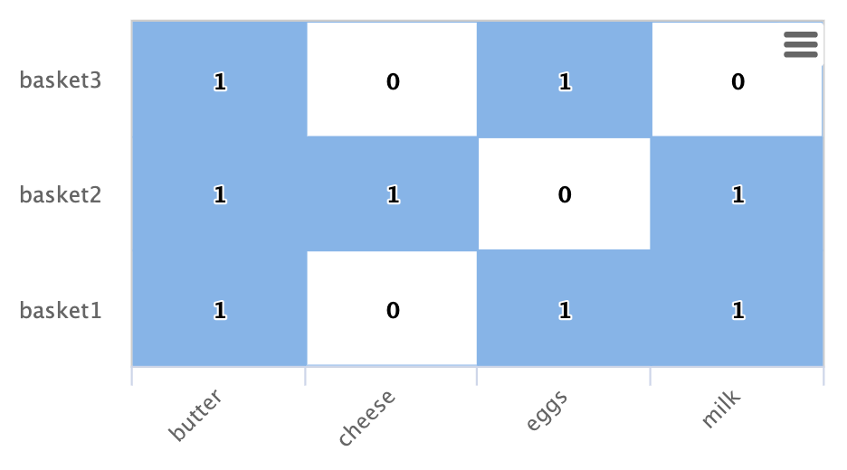
If we compute the dot product between the butter column and the other product columns you will find that the dot product equals the inbound degree in each case. This tells us that a nearest neighbor search, using a maximum inner product similarity, would select the column with the highest inbound degree.
Limiting Basket Out-Degree
The recommendation can be made stronger by limiting the out-degree of the baskets. The out-degree is the number of outbound links of a node in a graph. In the shopping basket example the outbound links from the baskets link to products. So limiting the out-degree will limit the size of the baskets.
Why does limiting the size of the shopping baskets make a stronger recommendation? To answer this question it helps to think about each shopping basket as voting for products that go with butter. In an election with two candidates if you were to vote for both candidates the votes would cancel each other out and have no effect. But if you vote for only one candidate your vote will affect the outcome. The same principle holds true for recommendations. As a basket votes for more products it dilutes the strength of its recommendation for any one product. A basket with just butter and one other item more strongly recommends that item.
The maxDocFreq parameter can be used to limit the graph "walk" to only include baskets that appear in the index a certain number of times.
Since each occurrence of a basket ID in the index is a link to a product, limiting the document frequency of the basket ID will limit the out-degree of the basket.
The maxDocFreq parameter is applied per shard.
If there is a single shard or documents are co-located by basket ID then the maxDocFreq will be an exact count.
Otherwise, it will return baskets with a max size of numShards * maxDocFreq.
The example below shows the maxDocFreq parameter applied to the nodes expression.
nodes(baskets,
      random(baskets, q="product_s:butter", fl="basket_s", rows="3"),
      walk="basket_s->basket_s",
      maxDocFreq="5",
      fq="-product_s:butter",
      gather="product_s",
      trackTraversal="true",
      count(*))
Node Scoring
The degree of the node describes how many nodes in the subgraph link to it. But this does not tell us if the node is particularly central to this subgraph or if it is just a very frequent node in the entire graph. Nodes that appear frequently in the subgraph but infrequently in the entire graph can be considered more relevant to the subgraph.
The search index contains information about how frequently each node appears in the entire index. Using a technique similar to tf-idf document scoring, graph expressions can combine the degree of the node with its inverse document frequency in the index to determine a relevancy score.
The scoreNodes function scores the nodes.
Below is an example of the scoreNodes function applied to the shopping basket node set.
scoreNodes(nodes(baskets,
                 random(baskets, q="product_s:butter", fl="basket_s", rows="3"),
                 walk="basket_s->basket_s",
                 fq="-product_s:butter",
                 gather="product_s",
                 trackTraversal="true",
                 count(*)))
The output now includes a nodeScore property.
In the output below notice how eggs has a higher nodeScore than milk even though they have the same count(*).
This is because milk appears more frequently in the entire index than eggs does.
The docFreq property added by the nodeScore function shows the document frequency in the index.
Because of the lower docFreq eggs is considered more relevant to this subgraph, and a better recommendation to be paired with butter.
{
  "result-set": {
    "docs": [
      {
        "node": "eggs",
        "nodeScore": 3.8930247,
        "field": "product_s",
        "numDocs": 10,
        "level": 1,
        "count(*)": 2,
        "collection": "baskets",
        "ancestors": [
          "basket1",
          "basket3"
        ],
        "docFreq": 2
      },
      {
        "node": "milk",
        "nodeScore": 3.0281217,
        "field": "product_s",
        "numDocs": 10,
        "level": 1,
        "count(*)": 2,
        "collection": "baskets",
        "ancestors": [
          "basket1",
          "basket2"
        ],
        "docFreq": 4
      },
      {
        "node": "cheese",
        "nodeScore": 2.7047482,
        "field": "product_s",
        "numDocs": 10,
        "level": 1,
        "count(*)": 1,
        "collection": "baskets",
        "ancestors": [
          "basket2"
        ],
        "docFreq": 1
      },
      {
        "EOF": true,
        "RESPONSE_TIME": 26
      }
    ]
  }
}
Temporal Graph Expressions
The examples above lay the groundwork for temporal graph queries.
Temporal graph queries allow the nodes function to walk the graph using windows of time
to surface cross-correlations within a temporal graph.
The nodes function currently supports graph walks using
ten second windows, daily windows and weekday windows.
Ten second windows are useful for event correlation and root cause analysis in log analytics. The daily and weekday windows are useful for correlating events that happen days apart.
In order to support temporal graph queries a truncated timestamp in ISO 8601 format must be added to the log records as a
string field at indexing time.
To support ten second time windows a ten second truncated timestamp should be indexed in a string field
as follows: 2021-02-10T20:51:30Z .
To support daily and weekly time windows a day truncated timestamp should be indexed in a string field as follows:
2021-02-10T00:00:00Z.
Solr’s indexing tool for Solr logs, described here, already adds the ten second truncated timestamps. So those using Solr to analyze Solr logs get temporal graph expressions for free.
Root Events
Once the ten second windows have been indexed with the log records we can devise a query that creates a set of root events. We can demonstrate this with an example using Solr log records.
In this example we’ll perform a Streaming Expression facet aggregation that finds the top 10, ten second windows with the highest average query time.
These time windows can be used to represent slow query events in a temporal graph query.
Here is the facet function:
facet(solr_logs, q="+type_s:query +distrib_s:false", buckets="time_ten_second_s", avg(qtime_i))Below is a snippet of the results with the 25 windows with the highest average query times:
{
  "result-set": {
    "docs": [
      {
        "avg(qtime_i)": 105961.38461538461,
        "time_ten_second_s": "2020-08-25T21:05:00Z"
      },
      {
        "avg(qtime_i)": 93150.16666666667,
        "time_ten_second_s": "2020-08-25T21:04:50Z"
      },
      {
        "avg(qtime_i)": 87742,
        "time_ten_second_s": "2020-08-25T21:04:40Z"
      },
      {
        "avg(qtime_i)": 72081.71929824562,
        "time_ten_second_s": "2020-08-25T21:05:20Z"
      },
      {
        "avg(qtime_i)": 62741.666666666664,
        "time_ten_second_s": "2020-08-25T12:30:20Z"
      },
      {
        "avg(qtime_i)": 56526,
        "time_ten_second_s": "2020-08-25T12:41:20Z"
      },
      ...

      {
        "avg(qtime_i)": 12893,
        "time_ten_second_s": "2020-08-25T17:28:10Z"
      },
      {
        "EOF": true,
        "RESPONSE_TIME": 34
      }
    ]
  }
}
Temporal Bipartite Subgraphs
Once we’ve identified a set of root events it’s easy to perform a graph query that creates a bipartite graph of the log events types that occurred within the same ten second windows.
With Solr logs there is a field called type_s which is the type of log event.
In order to see what log events happened in the same ten second window of our root events we can "walk" the ten second windows and gather the type_s field.
nodes(solr_logs,
      facet(solr_logs,
            q="+type_s:query +distrib_s:false",
            buckets="time_ten_second_s",
            avg(qtime_i)),
      walk="time_ten_second_s->time_ten_second_s",
      gather="type_s",
      count(*))
Below is the resulting node set:
{

  "result-set": {
    "docs": [
      {
        "node": "query",
        "count(*)": 10,
        "collection": "solr_logs",
        "field": "type_s",
        "level": 1
      },
      {
        "node": "admin",
        "count(*)": 2,
        "collection": "solr_logs",
        "field": "type_s",
        "level": 1
      },
      {
        "node": "other",
        "count(*)": 3,
        "collection": "solr_logs",
        "field": "type_s",
        "level": 1
      },
      {
        "node": "update",
        "count(*)": 2,
        "collection": "solr_logs",
        "field": "type_s",
        "level": 1
      },
      {
        "node": "error",
        "count(*)": 1,
        "collection": "solr_logs",
        "field": "type_s",
        "level": 1
      },
      {
        "EOF": true,
        "RESPONSE_TIME": 50
      }
    ]
  }
}
In this result set the node field holds the type of log events that occurred within the same ten second windows as the root events.
Notice that the event types include: query, admin, update and error.
The count(*) shows the degree centrality of the different log event types.
Notice that there is only one error event within the same ten second windows of the slow query events.
Window Parameter
For event correlation and root cause analysis it’s not enough to find events that occur within the same ten second root event windows.
What’s needed is to find events that occur within a window of time prior to each root event.
The window parameter allows you to specify this prior window of time as part of the query.
The window parameter is an integer which specifies the number of ten second time windows,
prior to each root event window, to include in the graph walk.
nodes(solr_logs,
      facet(solr_logs,
            q="+type_s:query +distrib_s:false",
            buckets="time_ten_second_s",
            avg(qtime_i)),
            walk="time_ten_second_s->time_ten_second_s",
      gather="type_s",
      window="-3",
      count(*))
Notice that the window parameter in this example is negative (-3). This will walk back in time from the events. A positive window will walk forward in time.
Below is the node set returned when the window parameter is added. Notice that there are now 29 error events within the 3 ten second windows prior to the slow query events.
{
  "result-set": {
    "docs": [
      {
        "node": "query",
        "count(*)": 62,
        "collection": "solr_logs",
        "field": "type_s",
        "level": 1
      },
      {
        "node": "admin",
        "count(*)": 41,
        "collection": "solr_logs",
        "field": "type_s",
        "level": 1
      },
      {
        "node": "other",
        "count(*)": 48,
        "collection": "solr_logs",
        "field": "type_s",
        "level": 1
      },
      {
        "node": "update",
        "count(*)": 11,
        "collection": "solr_logs",
        "field": "type_s",
        "level": 1
      },
      {
        "node": "error",
        "count(*)": 29,
        "collection": "solr_logs",
        "field": "type_s",
        "level": 1
      },
      {
        "EOF": true,
        "RESPONSE_TIME": 117
      }
    ]
  }
}
Degree as a Representation of Correlation
By performing link analysis on the temporal bipartite graph we can calculate the degree of each event type that occurs in the specified time windows. We established in the bipartite graph recommender example the direct relationship between inbound degree and the dot product. In the field of digital signal processing the dot product is used to represent correlation. In our temporal graph queries we can then view the inbound degree as a representation of correlation between the root events and the events that occur within the specified time windows.
Lag Parameter
Understanding the lag in the correlation is important for certain use cases. In a lagged correlation an event occurs and following a delay another event occurs. The window parameter doesn’t capture the delay as we only know that an event occurred somewhere within a prior window.
The lag parameter can be used to start calculating the window parameter a number of ten second windows in the past.
For example we could walk the graph in 20 second windows starting from 30 seconds prior to a set of root events.
By adjusting the lag and re-running the query we can determine which lagged window has the highest degree.
From this we can determine the delay.
Node Scoring and Temporal Anomaly Detection
The concept of node scoring can be applied to temporal graph queries to find events that are both correlated with a set of root events and anomalous to the root events. The degree calculation establishes the correlation between events but it does not establish if the event is a very common occurrence in the entire graph or specific to the subgraph.
The scoreNodes functions can be applied to score the nodes based on the degree and the commonality of the node’s term in the index.
This will establish whether the event is anomalous to the root events.
scoreNodes(nodes(solr_logs,
                 facet(solr_logs,
                       q="+type_s:query +distrib_s:false",
                       buckets="time_ten_second_s",
                       avg(qtime_i)),
                 walk="time_ten_second_s->time_ten_second_s",
                 gather="type_s",
                 window="-3",
                 count(*)))
Below is the node set once the scoreNodes function is applied.
Now we see that the highest scoring node is the error event.
This score give us a good indication of where to begin our root cause analysis.
{
  "result-set": {
    "docs": [
      {
        "node": "other",
        "nodeScore": 23.441727,
        "field": "type_s",
        "numDocs": 4513625,
        "level": 1,
        "count(*)": 48,
        "collection": "solr_logs",
        "docFreq": 99737
      },
      {
        "node": "query",
        "nodeScore": 16.957537,
        "field": "type_s",
        "numDocs": 4513625,
        "level": 1,
        "count(*)": 62,
        "collection": "solr_logs",
        "docFreq": 449189
      },
      {
        "node": "admin",
        "nodeScore": 22.829023,
        "field": "type_s",
        "numDocs": 4513625,
        "level": 1,
        "count(*)": 41,
        "collection": "solr_logs",
        "docFreq": 96698
      },
      {
        "node": "update",
        "nodeScore": 3.9480786,
        "field": "type_s",
        "numDocs": 4513625,
        "level": 1,
        "count(*)": 11,
        "collection": "solr_logs",
        "docFreq": 3838884
      },
      {
        "node": "error",
        "nodeScore": 26.62394,
        "field": "type_s",
        "numDocs": 4513625,
        "level": 1,
        "count(*)": 29,
        "collection": "solr_logs",
        "docFreq": 27622
      },
      {
        "EOF": true,
        "RESPONSE_TIME": 124
      }
    ]
  }
}
DAY and WEEKDAY Time Windows
To switch to day or weekday time windows we must first index day truncated ISO 8601 timestamps in a string field with the log records.
In the example below the field time_day_s contains the day truncated time stamps.
Then its simply a matter of specifying -3DAYS in the window parameter. This will switch from the default ten second time windows to daily windows.
scoreNodes(nodes(solr_logs,
                 facet(solr_logs,
                       q="+type_s:query +distrib_s:false",
                       buckets="time_day_s",
                       avg(qtime_i)),
                 walk="time_day_s->time_day_s",
                 gather="type_s",
                 window="-3DAYS",
                 count(*)))
There are times when you may need to skip the weekends when walking forwards or backwards in time. This is useful for correlating financial instruments that trade on weekdays. The WEEKDAYS time window will walk forward or backward the specified number of weekdays.
scoreNodes(nodes(solr_logs,
                 facet(solr_logs,
                       q="+type_s:query +distrib_s:false",
                       buckets="time_day_s",
                       avg(qtime_i)),
                 walk="time_day_s->time_day_s",
                 gather="type_s",
                 window="-3WEEKDAYS",
                 count(*)))