Interpolation, Derivatives and Integrals
This section explores the interrelated math expressions for interpolation and numerical calculus.
Interpolation
Interpolation is used to construct new data points between a set of known control of points. The ability to predict new data points allows for sampling along the curve defined by the control points.
The interpolation functions described below all return an interpolation function that can be passed to other functions which make use of the sampling capability.
If returned directly the interpolation function returns an array containing predictions for each of the control points.
This is useful in the case of loess interpolation which first smooths the control points and then interpolates the smoothed points.
All other interpolation functions simply return the original control points because interpolation predicts a curve that passes through the original control points.
There are different algorithms for interpolation that will result in different predictions along the curve. The math expressions library currently supports the following interpolation functions:
-
lerp: Linear interpolation predicts points that pass through each control point and form straight lines between control points. -
spline: Spline interpolation predicts points that pass through each control point and form a smooth curve between control points. -
akima: Akima spline interpolation is similar to spline interpolation but is stable to outliers. -
loess: Loess interpolation first performs a non-linear local regression to smooth the original control points. Then a spline is used to interpolate the smoothed control points.
Sampling Along the Curve
One way to better understand interpolation is to visualize what it means to sample along a curve. The example below zooms in on a specific region of a curve by sampling the curve between a specific x-axis range.
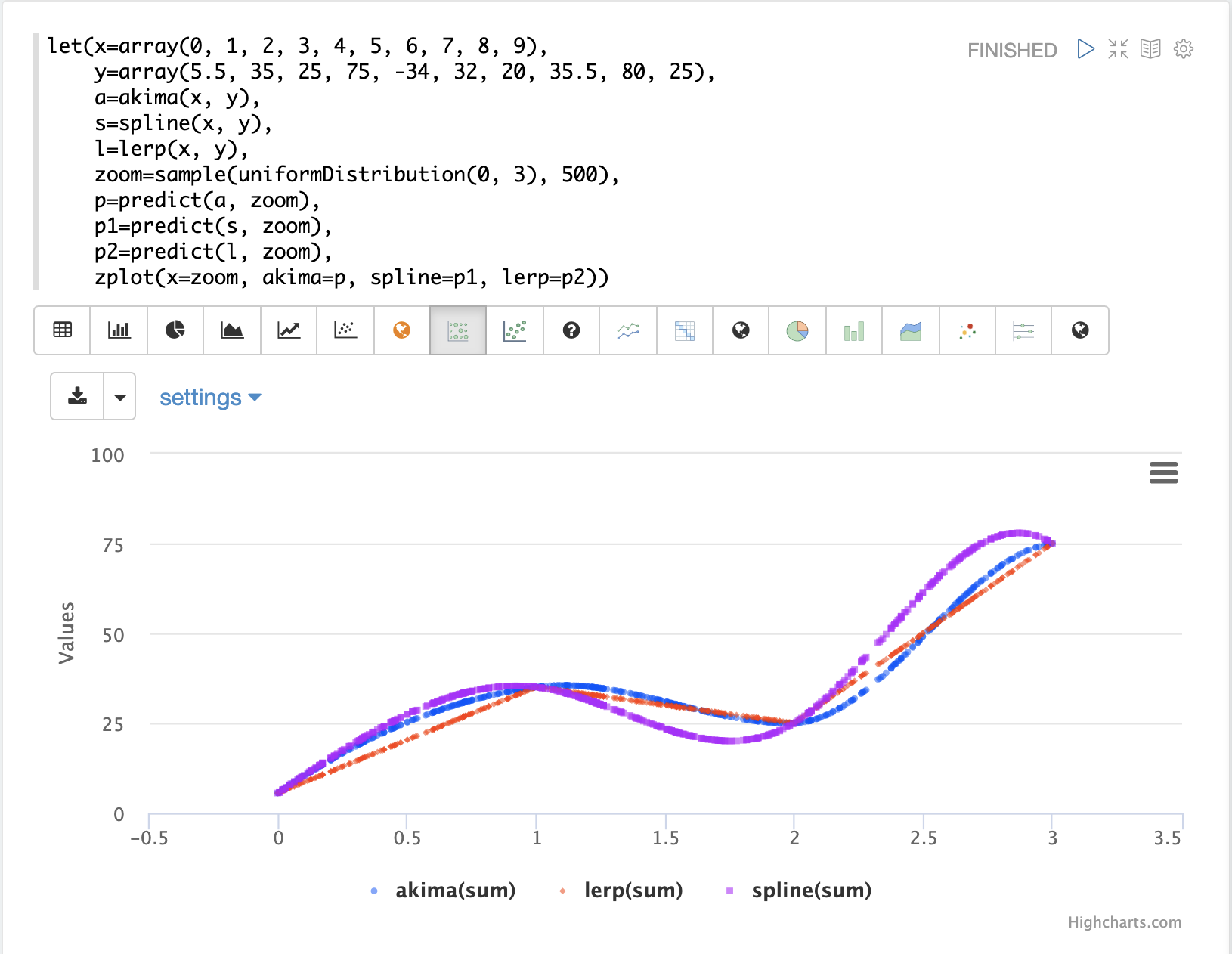
The visualization above first creates two arrays with x and y-axis points.
Notice that the x-axis ranges from 0 to 9.
Then the akima, spline and lerp functions are applied to the vectors to create three interpolation functions.
Then 500 hundred random samples are drawn from a uniform distribution between 0 and 3. These are the new zoomed in x-axis points, between 0 and 3. Notice that we are sampling a specific area of the curve.
Then the predict function is used to predict y-axis points for the sampled x-axis, for all three interpolation functions.
Finally all three prediction vectors are plotted with the sampled x-axis points.
The red line is the lerp interpolation, the blue line is the akima and the purple line is the spline interpolation.
You can see they each produce different curves in between the control points.
Smoothing Interpolation
The loess function is a smoothing interpolator which means it doesn’t derive a function that passes through the original control points.
Instead the loess function returns a function that smooths the original control points.
A technique known as local regression is used to compute the smoothed curve. The size of the neighborhood of the local regression can be adjusted to control how close the new curve conforms to the original control points.
The loess function is passed x- and y-axes and fits a smooth curve to the data.
If only a single array is provided it is treated as the y-axis and a sequence is generated for the x-axis.
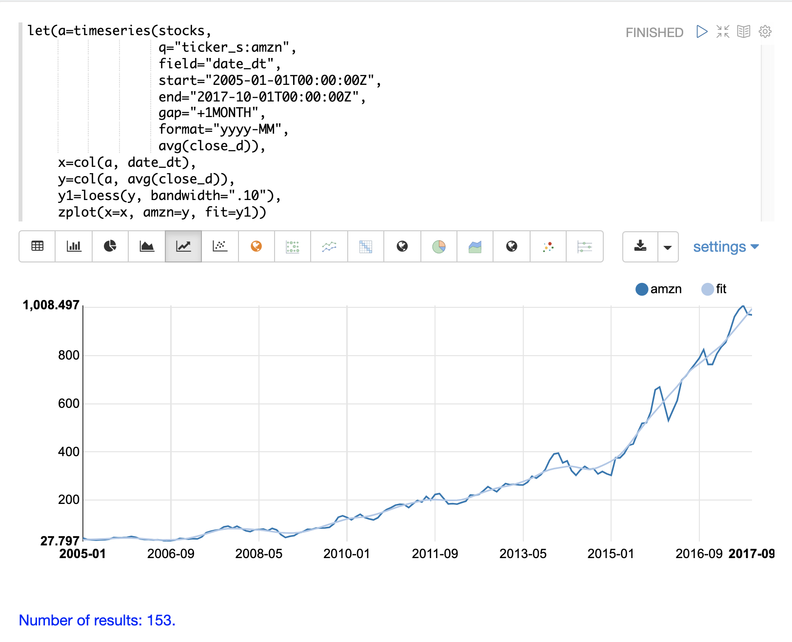
The example below shows the loess function being used to model a monthly time series.
In the example the timeseries function is used to generate a monthly time series of average closing prices for the stock ticker AMZN.
The date_dt and avg(close_d) fields from the time series are then vectorized and stored in variables x and y.
The loess function is then applied to the y vector containing the average closing prices.
The bandwidth named parameter specifies the percentage of the data set used to compute the local regression.
The loess function returns the fitted model of smoothed data points.
The zplot function is then used to plot the x, y and y1 variables.
Derivatives
The derivative of a function measures the rate of change of the y value in respect to the rate of change of the x value.
The derivative function can compute the derivative for any of the interpolation functions described above.
Each interpolation function will produce different derivatives that match the characteristics of the function.
The First Derivative (Velocity)
A simple example shows how the derivative function is used to calculate the rate of change or velocity.
In the example two vectors are created, one representing hours and one representing miles traveled.
The lerp function is then used to create a linear interpolation of the hours and miles vectors.
The derivative function is then applied to the linear interpolation.
zplot is then used to plot the hours on the x-axis and miles on the y-axis, and the derivative as mph, at each x-axis point.
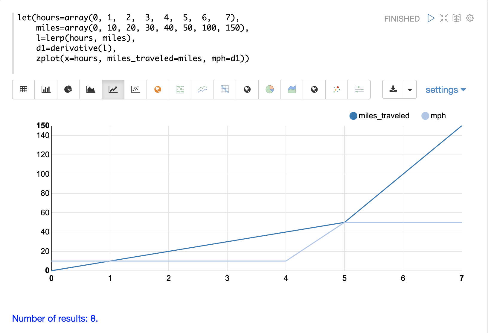
Notice that the miles_traveled line has a slope of 10 until the 5th hour where it changes to a slope of 50. The mph line, which is the derivative, visualizes the velocity of the miles_traveled line.
Also notice that the derivative is calculated along straight lines showing immediate change from one point to the next.
This is because linear interpolation (lerp) is used as the interpolation function.
If the spline or akima functions had been used it would have produced a derivative with rounded curves.
The Second Derivative (Acceleration)
While the first derivative represents velocity, the second derivative represents acceleration.
The second the derivative is the derivative of the first derivative.
The example below builds on the first example and adds the second derivative.
Notice that the second derivative d2 is taken by applying the derivative function to a linear interpolation of the first derivative.
The second derivative is plotted as acceleration on the chart.
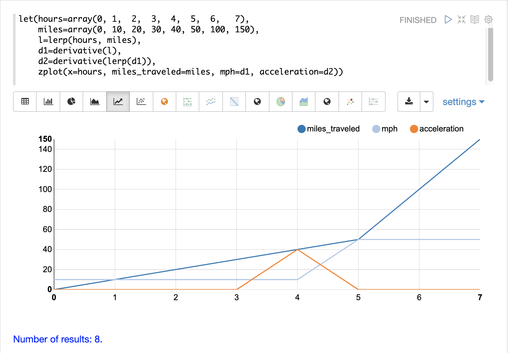
Notice that the acceleration line is 0 until the mph line increases from 10 to 50. At this point the acceleration line moves to 40. As the mph line stays at 50, the acceleration line drops to 0.
Price Velocity
The example below shows how to plot the derivative for a time series generated by the timeseries function.
In the example a monthly time series is generated for the average closing price for the stock ticker amzn.
The avg(close) column is vectorized and interpolated using linear interpolation (lerp).
The zplot function is then used to plot the derivative of the time series.
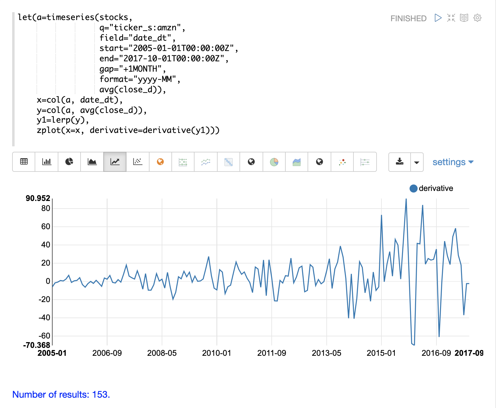
Notice that the derivative plot clearly shows the rates of change in the stock price over time.
Integrals
An integral is a measure of the volume underneath a curve.
The integral function computes the cumulative integrals for a curve or the integral for a specific range of an interpolated curve.
Like the derivative function the integral function operates over interpolation functions.
Single Integral
If the integral function is passed a start and end range it will compute the volume under the curve within that specific range.
In the example below the integral function computes an integral for the entire range of the curve, 0 through 10.
Notice that the integral function is passed the interpolated curve and the start and end range, and returns the integral for the range.
let(x=array(0, 1, 2, 3, 4, 5, 6, 7, 8, 9, 10, 11, 12, 13, 14, 15, 16, 17, 18, 19, 20),
    y=array(0, 1, 2, 3, 4, 5.7, 6, 7, 7, 7,6, 7, 7, 7, 6, 5, 5, 3, 2, 1, 0),
    curve=loess(x, y, bandwidth=.3),
    integral=integral(curve,  0, 10))
When this expression is sent to the /stream handler it responds with:
{
  "result-set": {
    "docs": [
      {
        "integral": 45.300912584519914
      },
      {
        "EOF": true,
        "RESPONSE_TIME": 0
      }
    ]
  }
}
Cumulative Integral Plot
If the integral function is passed a single interpolated curve it returns a vector of the cumulative integrals for the curve.
The cumulative integrals vector contains a cumulative integral calculation for each x-axis point.
The cumulative integral is calculated by taking the integral of the range between each x-axis point and the first x-axis point.
In the example above this would mean calculating a vector of integrals as such:
let(x=array(0, 1, 2, 3, 4, 5, 6, 7, 8, 9, 10, 11, 12, 13, 14, 15, 16, 17, 18, 19, 20),
    y=array(0, 1, 2, 3, 4, 5.7, 6, 7, 7, 7,6, 7, 7, 7, 6, 5, 5, 3, 2, 1, 0),
    curve=loess(x, y, bandwidth=.3),
    integrals=array(0, integral(curve, 0, 1), integral(curve, 0, 2), integral(curve, 0, 3), ...)
The plot of cumulative integrals visualizes how much cumulative volume of the curve is under each point x-axis point.
The example below shows the cumulative integral plot for a time series generated by the timeseries function.
In the example a monthly time series is generated for the average closing price for the stock ticker amzn.
The avg(close) column is vectorized and interpolated using a spline.
The zplot function is then used to plot the cumulative integral of the time series.
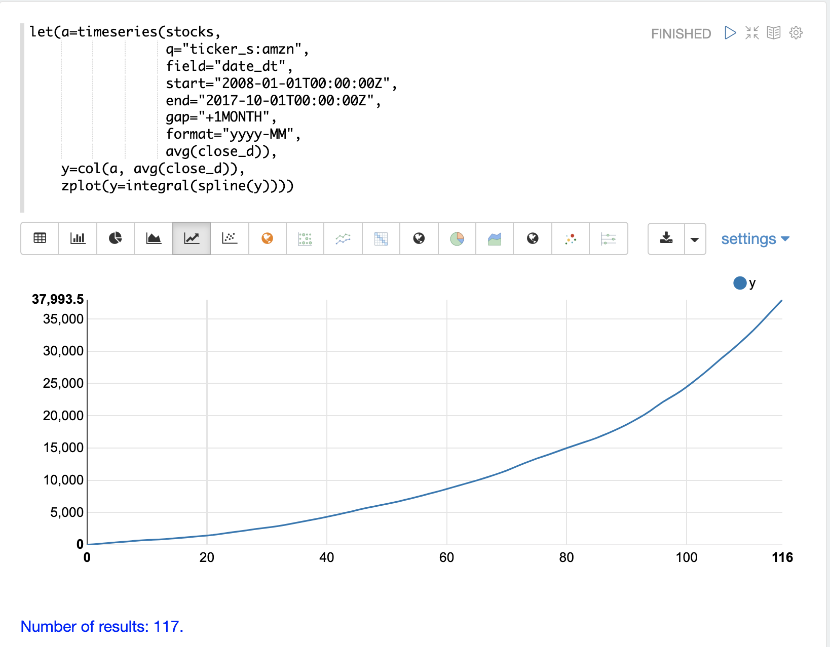
The plot above visualizes the volume under the curve as the AMZN stock price changes over time. Because this plot is cumulative, the volume under a stock price time series which stays the same over time, will have a positive linear slope. A stock that has rising prices will have a concave shape and a stock with falling prices will have a convex shape.
In this particular example the integral plot becomes more concave over time showing accelerating increases in stock price.
Bicubic Spline
The bicubicSpline function can be used to interpolate and predict values anywhere within a grid of data.
A simple example will make this more clear:
let(years=array(1998, 2000, 2002, 2004, 2006),
    floors=array(1, 5, 9, 13, 17, 19),
    prices = matrix(array(300000, 320000, 330000, 350000, 360000, 370000),
                    array(320000, 330000, 340000, 350000, 365000, 380000),
                    array(400000, 410000, 415000, 425000, 430000, 440000),
                    array(410000, 420000, 425000, 435000, 445000, 450000),
                    array(420000, 430000, 435000, 445000, 450000, 470000)),
    bspline=bicubicSpline(years, floors, prices),
    prediction=predict(bspline, 2003, 8))
In this example a bicubic spline is used to interpolate a matrix of real estate data.
Each row of the matrix represent specific years.
Each column of the matrix represents floors of the building.
The grid of numbers is the average selling price of an apartment for each year and floor.
For example in 2002 the average selling price for the 9th floor was 415000 (row 3, column 3).
The bicubicSpline function is then used to interpolate the grid, and the predict function is used to predict a value for year 2003, floor 8.
Notice that the matrix does not include a data point for year 2003, floor 8.
The bicubicSpline function creates that data point based on the surrounding data in the matrix:
{
  "result-set": {
    "docs": [
      {
        "prediction": 418279.5009328358
      },
      {
        "EOF": true,
        "RESPONSE_TIME": 0
      }
    ]
  }
}