This section of the user guide explores functions that are commonly used in the field of Digital Signal Processing (DSP).
Dot Product
The dotProduct function is used to calculate the dot product of two arrays.
The dot product is a fundamental calculation for the DSP functions discussed in this section. Before diving into
the more advanced DSP functions, its useful to get a better understanding of how the dot product calculation works.
Combining Two Arrays
The dotProduct function can be used to combine two arrays into a single product. A simple example can help
illustrate this concept.
In the example below two arrays are set to variables a and b and then operated on by the dotProduct function.
The output of the dotProduct function is set to variable c.
Then the mean function is then used to compute the mean of the first array which is set to the variable d.
Both the dot product and the mean are included in the output.
When we look at the output of this expression we see that the dot product and the mean of the first array are both 30.
The dotProduct function calculated the mean of the first array.
let(echo="c, d",
    a=array(10, 20, 30, 40, 50),
    b=array(.2, .2, .2, .2, .2),
    c=dotProduct(a, b),
    d=mean(a))
When this expression is sent to the /stream handler it responds with:
{
  "result-set": {
    "docs": [
      {
        "c": 30,
        "d": 30
      },
      {
        "EOF": true,
        "RESPONSE_TIME": 0
      }
    ]
  }
}
To get a better understanding of how the dot product calculated the mean we can perform the steps of the calculation using vector math and look at the output of each step.
In the example below the ebeMultiply function performs an element-by-element multiplication of
two arrays. This is the first step of the dot product calculation. The result of the element-by-element
multiplication is assigned to variable c.
In the next step the add function adds all the elements of the array in variable c.
Notice that multiplying each element of the first array by .2 and then adding the results is equivalent to the formula for computing the mean of the first array. The formula for computing the mean of an array is to add all the elements and divide by the number of elements.
The output includes the output of both the ebeMultiply function and the add function.
let(echo="c, d",
    a=array(10, 20, 30, 40, 50),
    b=array(.2, .2, .2, .2, .2),
    c=ebeMultiply(a, b),
    d=add(c))
When this expression is sent to the /stream handler it responds with:
{
  "result-set": {
    "docs": [
      {
        "c": [
          2,
          4,
          6,
          8,
          10
        ],
        "d": 30
      },
      {
        "EOF": true,
        "RESPONSE_TIME": 0
      }
    ]
  }
}
In the example above two arrays were combined in a way that produced the mean of the first. In the second array each value was set to ".2". Another way of looking at this is that each value in the second array has the same weight. By varying the weights in the second array we can produce a different result. For example if the first array represents a time series, the weights in the second array can be set to add more weight to a particular element in the first array.
The example below creates a weighted average with the weight decreasing from right to left. Notice that the weighted mean of 36.666 is larger than the previous mean which was 30. This is because more weight was given to last element in the array.
let(echo="c, d",
    a=array(10, 20, 30, 40, 50),
    b=array(.066666666666666,.133333333333333,.2, .266666666666666, .33333333333333),
    c=ebeMultiply(a, b),
    d=add(c))
When this expression is sent to the /stream handler it responds with:
{
  "result-set": {
    "docs": [
      {
        "c": [
          0.66666666666666,
          2.66666666666666,
          6,
          10.66666666666664,
          16.6666666666665
        ],
        "d": 36.66666666666646
      },
      {
        "EOF": true,
        "RESPONSE_TIME": 0
      }
    ]
  }
}
Representing Correlation
Often when we think of correlation, we are thinking of Pearson correlation in the field of statistics. But the definition of correlation is actually more general: a mutual relationship or connection between two or more things. In the field of digital signal processing the dot product is used to represent correlation. The examples below demonstrates how the dot product can be used to represent correlation.
In the example below the dot product is computed for two vectors. Notice that the vectors have different values that fluctuate together. The output of the dot product is 190, which is hard to reason about because it’s not scaled.
let(echo="c, d",
    a=array(10, 20, 30, 20, 10),
    b=array(1, 2, 3, 2, 1),
    c=dotProduct(a, b))
When this expression is sent to the /stream handler it responds with:
{
  "result-set": {
    "docs": [
      {
        "c": 190
      },
      {
        "EOF": true,
        "RESPONSE_TIME": 0
      }
    ]
  }
}
One approach to scaling the dot product is to first scale the vectors so that both vectors have a magnitude of 1. Vectors with a
magnitude of 1, also called unit vectors, are used when comparing only the angle between vectors rather then the magnitude.
The unitize function can be used to unitize the vectors before calculating the dot product.
Notice in the example below the dot product result, set to variable e, is effectively 1. When applied to unit vectors the dot product
will be scaled between 1 and -1. Also notice in the example cosineSimilarity is calculated on the unscaled vectors and the
answer is also effectively 1. This is because cosine similarity is a scaled dot product.
let(echo="e, f",
    a=array(10, 20, 30, 20, 10),
    b=array(1, 2, 3, 2, 1),
    c=unitize(a),
    d=unitize(b),
    e=dotProduct(c, d),
    f=cosineSimilarity(a, b))
When this expression is sent to the /stream handler it responds with:
{
  "result-set": {
    "docs": [
      {
        "e": 0.9999999999999998,
        "f": 0.9999999999999999
      },
      {
        "EOF": true,
        "RESPONSE_TIME": 0
      }
    ]
  }
}
If we transpose the first two numbers in the first array, so that the vectors are not perfectly correlated, we see that the cosine similarity drops. This illustrates how the dot product represents correlation.
let(echo="c, d",
    a=array(20, 10, 30, 20, 10),
    b=array(1, 2, 3, 2, 1),
    c=cosineSimilarity(a, b))
When this expression is sent to the /stream handler it responds with:
{
  "result-set": {
    "docs": [
      {
        "c": 0.9473684210526314
      },
      {
        "EOF": true,
        "RESPONSE_TIME": 0
      }
    ]
  }
}
Convolution
The conv function calculates the convolution of two vectors. The convolution is calculated by reversing
the second vector and sliding it across the first vector. The dot product of the two vectors
is calculated at each point as the second vector is slid across the first vector.
The dot products are collected in a third vector which is the convolution of the two vectors.
Moving Average Function
Before looking at an example of convolution its useful to review the movingAvg function. The moving average
function computes a moving average by sliding a window across a vector and computing
the average of the window at each shift. If that sounds similar to convolution, that’s because the movingAvg function
is syntactic sugar for convolution.
Below is an example of a moving average with a window size of 5. Notice that original vector has 13 elements
but the result of the moving average has only 9 elements. This is because the movingAvg function
only begins generating results when it has a full window. In this case because the window size is 5 so the
moving average starts generating results from the 4th index of the original array.
let(a=array(1, 2, 3, 4, 5, 6, 7, 6, 5, 4, 3, 2, 1),
    b=movingAvg(a, 5))
When this expression is sent to the /stream handler it responds with:
{
  "result-set": {
    "docs": [
      {
        "b": [
          3,
          4,
          5,
          5.6,
          5.8,
          5.6,
          5,
          4,
          3
        ]
      },
      {
        "EOF": true,
        "RESPONSE_TIME": 0
      }
    ]
  }
}
Convolutional Smoothing
The moving average can also be computed using convolution. In the example
below the conv function is used to compute the moving average of the first array
by applying the second array as the filter.
Looking at the result, we see that it is not exactly the same as the result
of the movingAvg function. That is because the conv pads zeros
to the front and back of the first vector so that the window size is always full.
let(a=array(1, 2, 3, 4, 5, 6, 7, 6, 5, 4, 3, 2, 1),
    b=array(.2, .2, .2, .2, .2),
    c=conv(a, b))
When this expression is sent to the /stream handler it responds with:
{
  "result-set": {
    "docs": [
      {
        "c": [
          0.2,
          0.6000000000000001,
          1.2,
          2.0000000000000004,
          3.0000000000000004,
          4,
          5,
          5.6000000000000005,
          5.800000000000001,
          5.6000000000000005,
          5.000000000000001,
          4,
          3,
          2,
          1.2000000000000002,
          0.6000000000000001,
          0.2
        ]
      },
      {
        "EOF": true,
        "RESPONSE_TIME": 0
      }
    ]
  }
}
We achieve the same result as the movingAvg function by using the copyOfRange function to copy a range of
the result that drops the first and last 4 values of
the convolution result. In the example below the precision function is also also used to remove floating point errors from the
convolution result. When this is added the output is exactly the same as the movingAvg function.
let(a=array(1, 2, 3, 4, 5, 6, 7, 6, 5, 4, 3, 2, 1),
    b=array(.2, .2, .2, .2, .2),
    c=conv(a, b),
    d=copyOfRange(c, 4, 13),
    e=precision(d, 2))
When this expression is sent to the /stream handler it responds with:
{
  "result-set": {
    "docs": [
      {
        "e": [
          3,
          4,
          5,
          5.6,
          5.8,
          5.6,
          5,
          4,
          3
        ]
      },
      {
        "EOF": true,
        "RESPONSE_TIME": 0
      }
    ]
  }
}
Cross-Correlation
Cross-correlation is used to determine the delay between two signals. This is accomplished by sliding one signal across another and calculating the dot product at each shift. The dot products are collected into a vector which represents the correlation at each shift. The highest dot product in the cross-correlation vector is the point where the two signals are most closely correlated.
The sliding dot product used in convolution can also be used to represent cross-correlation between two vectors. The only difference in the formula when representing correlation is that the second vector is not reversed.
Notice in the example below that the second vector is reversed by the rev function before it is operated on by the conv function.
The conv function reverses the second vector so it will be flipped back to its original order to perform the correlation calculation
rather then the convolution calculation.
Notice in the result the highest value is 217. This is the point where the two vectors have the highest correlation.
let(a=array(1, 2, 3, 4, 5, 6, 7, 6, 5, 4, 3, 2, 1),
    b=array(4, 5, 6, 7, 6, 5, 4, 3, 2, 1),
    c=conv(a, rev(b)))
When this expression is sent to the /stream handler it responds with:
{
  "result-set": {
    "docs": [
      {
        "c": [
          1,
          4,
          10,
          20,
          35,
          56,
          84,
          116,
          149,
          180,
          203,
          216,
          217,
          204,
          180,
          148,
          111,
          78,
          50,
          28,
          13,
          4
        ]
      },
      {
        "EOF": true,
        "RESPONSE_TIME": 0
      }
    ]
  }
}
Find Delay
It is fairly simple to compute the delay from the cross-correlation result, but a convenience function called finddelay can
be used to find the delay directly. Under the covers finddelay uses convolutional math to compute the cross-correlation vector
and then computes the delay between the two signals.
Below is an example of the finddelay function. Notice that the finddelay function reports a 3 period delay between the first
and second signal.
let(a=array(1, 2, 3, 4, 5, 6, 7, 6, 5, 4, 3, 2, 1),
    b=array(4, 5, 6, 7, 6, 5, 4, 3, 2, 1),
    c=finddelay(a, b))
When this expression is sent to the /stream handler it responds with:
{
  "result-set": {
    "docs": [
      {
        "c": 3
      },
      {
        "EOF": true,
        "RESPONSE_TIME": 0
      }
    ]
  }
}
Autocorrelation
Autocorrelation measures the degree to which a signal is correlated with itself. Autocorrelation is used to determine if a vector contains a signal or is purely random.
A few examples, with plots, will help to understand the concepts.
In the first example the sin function is wrapped around a sequence function to generate a sine wave. The result of this
is plotted in the image below. Notice that there is a structure to the plot that is clearly not random.
sin(sequence(256, 0, 6))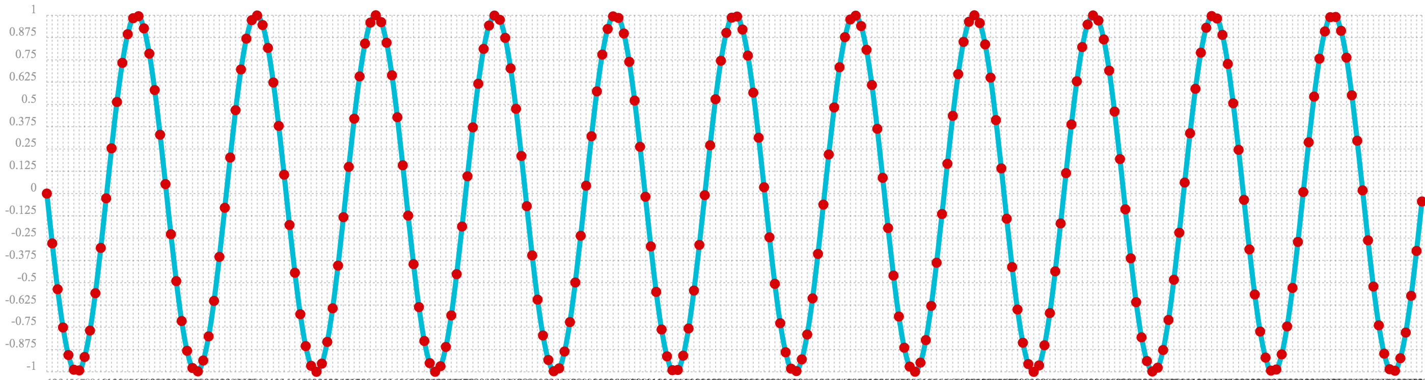
In the next example the sample function is used to draw 256 samples from a uniformDistribution to create a
vector of random data. The result of this is plotted in the image below. Notice that there is no clear structure to the
data and the data appears to be random.
sample(uniformDistribution(-1.5, 1.5), 256)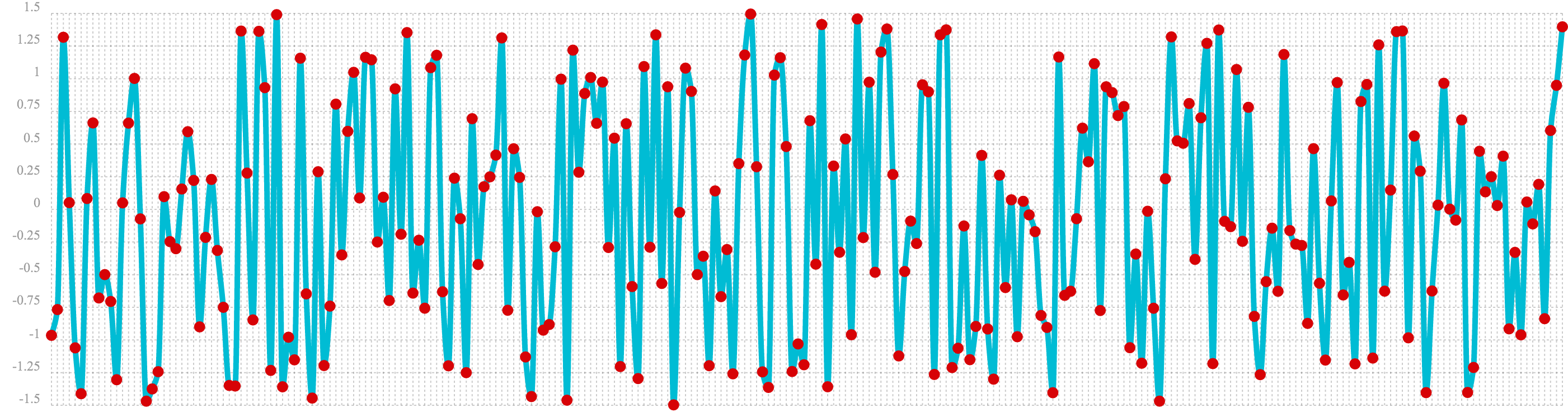
In the next example the random noise is added to the sine wave using the ebeAdd function.
The result of this is plotted in the image below. Notice that the sine wave has been hidden
somewhat within the noise. Its difficult to say for sure if there is structure. As plots
becomes more dense it can become harder to see a pattern hidden within noise.
let(a=sin(sequence(256, 0, 6)),
    b=sample(uniformDistribution(-1.5, 1.5), 256),
    c=ebeAdd(a, b))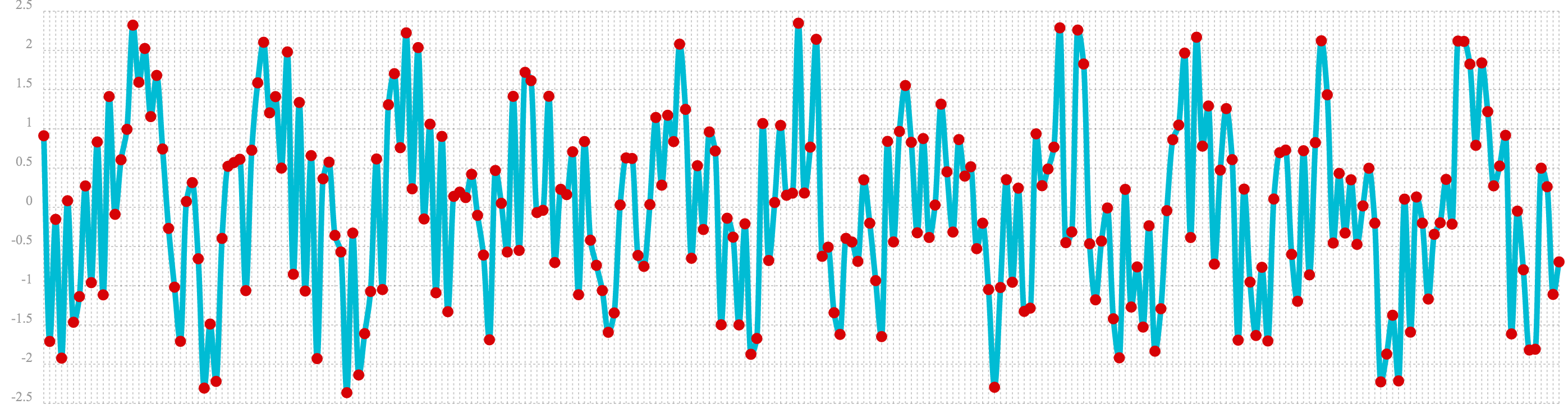
In the next examples autocorrelation is performed with each of the vectors shown above to see what the autocorrelation plots look like.
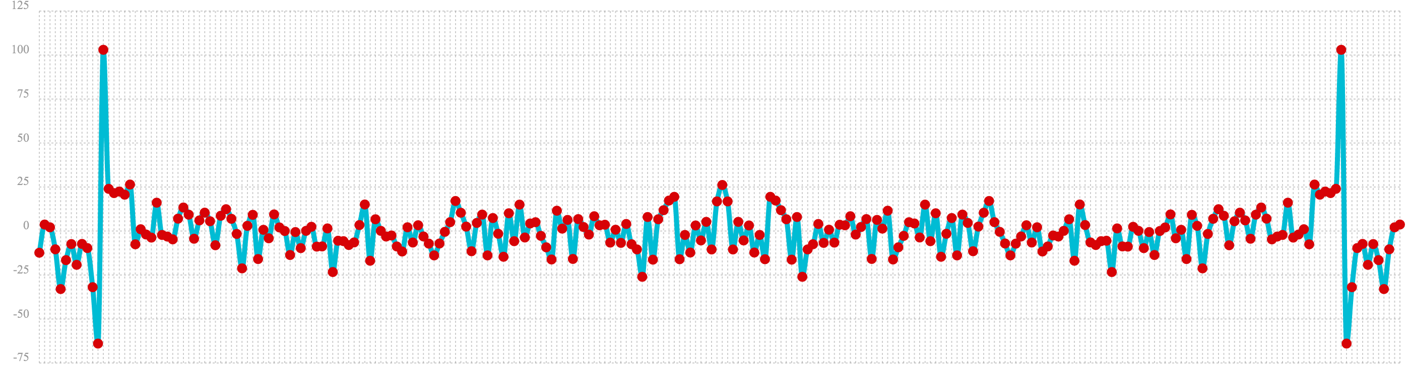
In the example below the conv function is used to autocorrelate the first vector which is the sine wave.
Notice that the conv function is simply correlating the sine wave with itself.
The plot has a very distinct structure to it. As the sine wave is slid across a copy of itself the correlation moves up and down in increasing intensity until it reaches a peak. This peak is directly in the center and is the the point where the sine waves are directly lined up. Following the peak the correlation moves up and down in decreasing intensity as the sine wave slides farther away from being directly lined up.
This is the autocorrelation plot of a pure signal.
let(a=sin(sequence(256, 0, 6)),
    b=conv(a, rev(a)),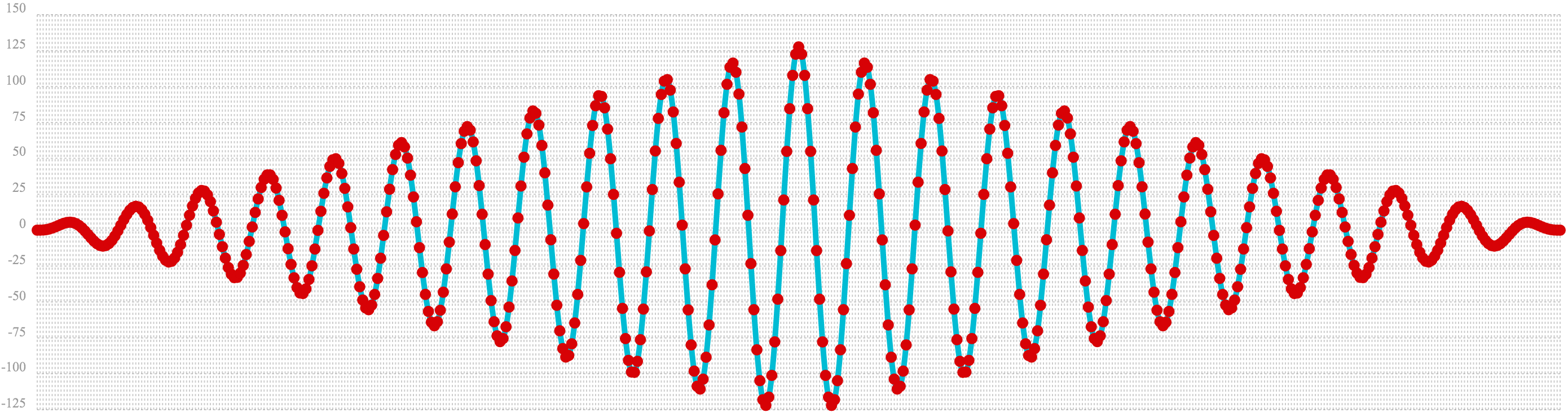
In the example below autocorrelation is performed with the vector of pure noise. Notice that the autocorrelation plot has a very different plot then the sine wave. In this plot there is long period of low intensity correlation that appears to be random. Then in the center a peak of high intensity correlation where the vectors are directly lined up. This is followed by another long period of low intensity correlation.
This is the autocorrelation plot of pure noise.
let(a=sample(uniformDistribution(-1.5, 1.5), 256),
    b=conv(a, rev(a)),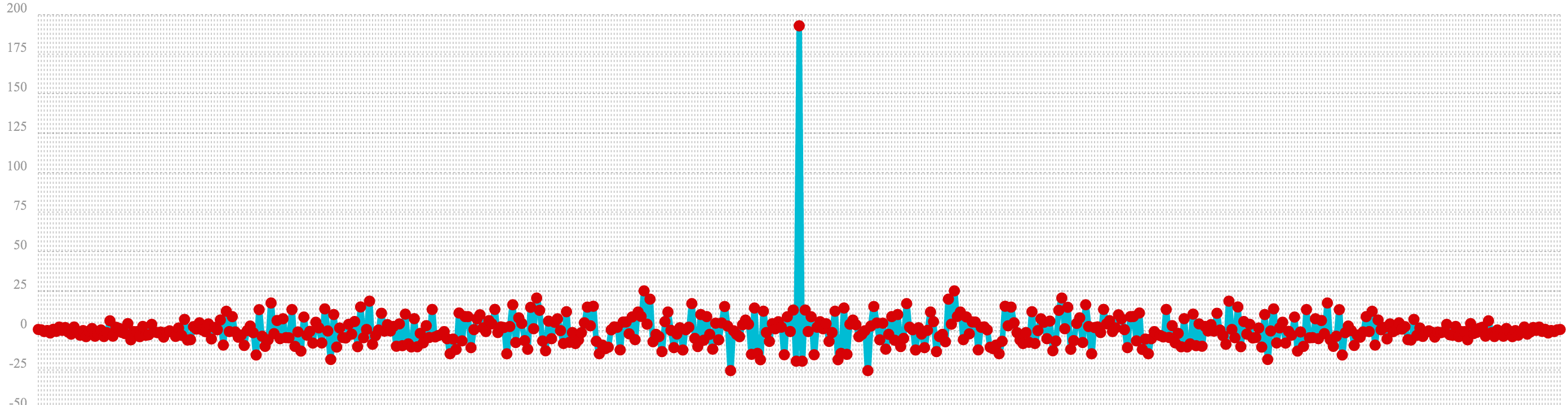
In the example below autocorrelation is performed on the vector with the sine wave hidden within the noise. Notice that this plot shows very clear signs of structure which is similar to autocorrelation plot of the pure signal. The correlation is less intense due to noise but the shape of the correlation plot suggests strongly that there is an underlying signal hidden within the noise.
let(a=sin(sequence(256, 0, 6)),
    b=sample(uniformDistribution(-1.5, 1.5), 256),
    c=ebeAdd(a, b),
    d=conv(c, rev(c))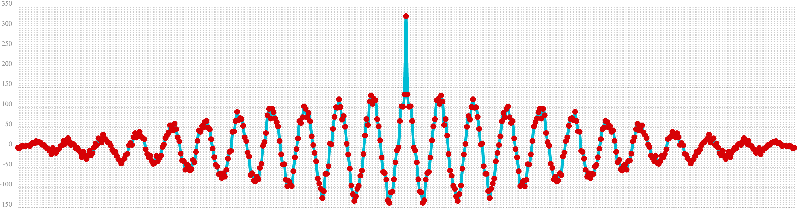
Discrete Fourier Transform
The convolution based functions described above are operating on signals in the time domain. In the time domain the X axis is time and the Y axis is the quantity of some value at a specific point in time.
The discrete Fourier Transform translates a time domain signal into the frequency domain. In the frequency domain the X axis is frequency, and Y axis is the accumulated power at a specific frequency.
The basic principle is that every time domain signal is composed of one or more signals (sine waves) at different frequencies. The discrete Fourier transform decomposes a time domain signal into its component frequencies and measures the power at each frequency.
The discrete Fourier transform has many important uses. In the example below, the discrete Fourier transform is used to determine if a signal has structure or if it is purely random.
Complex Result
The fft function performs the discrete Fourier Transform on a vector of real data. The result
of the fft function is returned as complex numbers. A complex number has two parts, real and imaginary.
The imaginary part of the complex number is ignored in the examples below, but there
are many tutorials on the FFT and that include complex numbers available online.
But before diving into the examples it is important to understand how the fft function formats the
complex numbers in the result.
The fft function returns a matrix with two rows. The first row in the matrix is the real
part of the complex result. The second row in the matrix is the imaginary part of the complex result.
The rowAt function can be used to access the rows so they can be processed as vectors.
This approach was taken because all of the vector math functions operate on vectors of real numbers.
Rather then introducing a complex number abstraction into the expression language, the fft result is
represented as two vectors of real numbers.
Fast Fourier Transform Examples
In the first example the fft function is called on the sine wave used in the autocorrelation example.
The results of the fft function is a matrix. The rowAt function is used to return the first row of
the matrix which is a vector containing the real values of the fft response.
The plot of the real values of the fft response is shown below. Notice there are two
peaks on opposite sides of the plot. The plot is actually showing a mirrored response. The right side
of the plot is an exact mirror of the left side. This is expected when the fft is run on real rather then
complex data.
Also notice that the fft has accumulated significant power in a single peak. This is the power associated with
the specific frequency of the sine wave. The vast majority of frequencies in the plot have close to 0 power
associated with them. This fft shows a clear signal with very low levels of noise.
let(a=sin(sequence(256, 0, 6)),
    b=fft(a),
    c=rowAt(b, 0))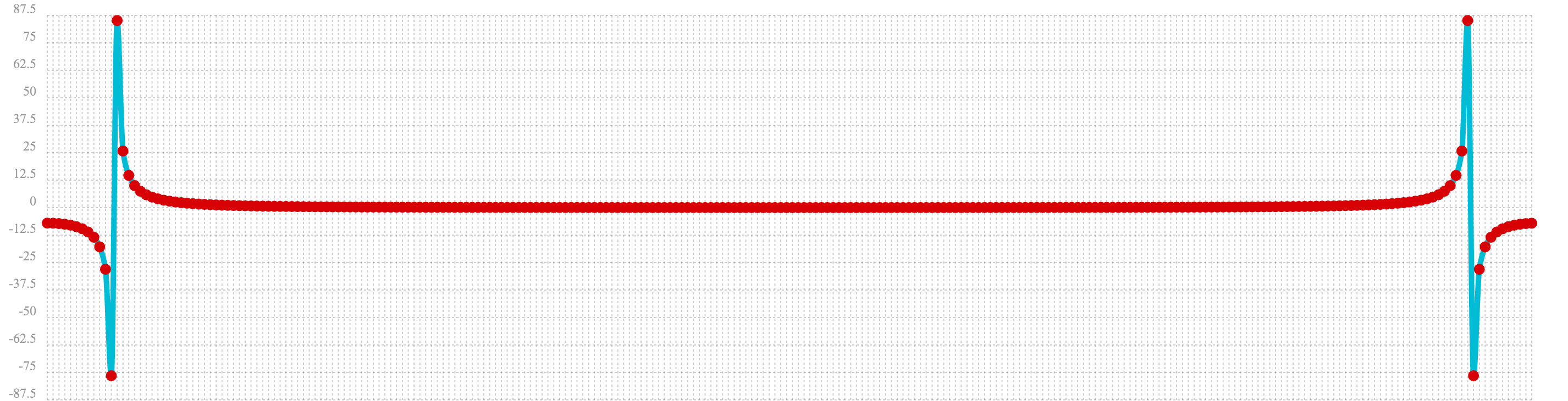
In the second example the fft function is called on a vector of random data similar to one used in the
autocorrelation example. The plot of the real values of the fft response is shown below.
Notice that in is this response there is no clear peak. Instead all frequencies have accumulated a random level of
power. This fft shows no clear sign of signal and appears to be noise.
let(a=sample(uniformDistribution(-1.5, 1.5), 256),
    b=fft(a),
    c=rowAt(b, 0))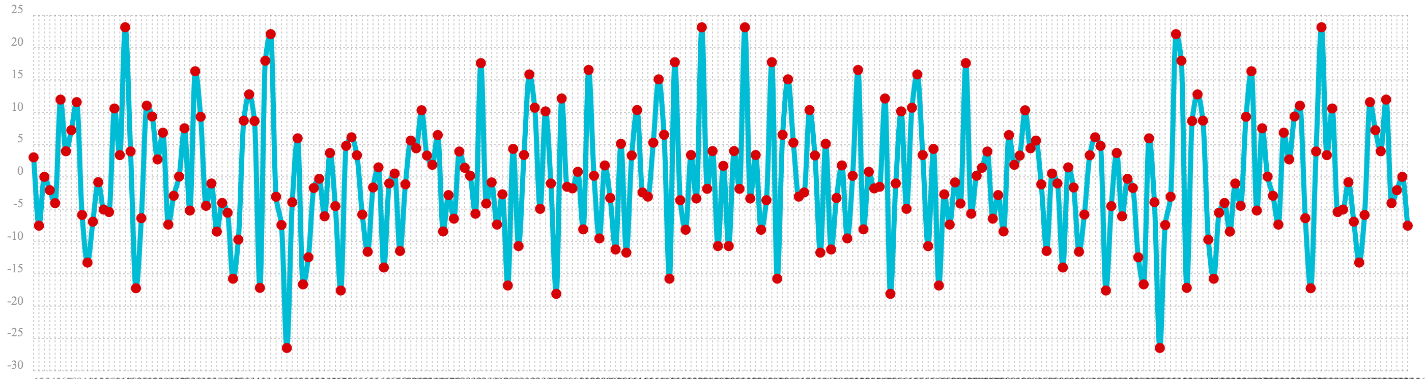
In the third example the fft function is called on the same signal hidden within noise that was used for
the autocorrelation example. The plot of the real values of the fft response is shown below.
Notice that there are two clear mirrored peaks, at the same locations as the fft of the pure signal. But
there is also now considerable noise on the frequencies. The fft has found the signal and but also
shows that there is considerable noise along with the signal.
let(a=sin(sequence(256, 0, 6)),
    b=sample(uniformDistribution(-1.5, 1.5), 256),
    c=ebeAdd(a, b),
    d=fft(c),
    e=rowAt(d, 0))